{
"cells": [
{
"cell_type": "markdown",
"metadata": {},
"source": [
"\n",
"\n"
]
},
{
"cell_type": "markdown",
"metadata": {},
"source": [
"# Getting started with DLProf\n",
"\n",
"**Contents of this notebook:**\n",
"\n",
"- [Introduction to DLProf](#Introduction-to-DLProf)\n",
"- [Profiling using DLProf](#Profiling-using-DLProf)\n",
"- [Visualising profiles using DLProfviewer](#Visualising-profiles-using-DLProfviewer)\n",
"- [Improving throughput using DLProf Expert system](#Improving-throughput-using-DLProf-Expert-system)\n",
"\n",
"\n",
"**By the End of this Notebook you will:**\n",
"\n",
"- Learn the basics of `dlProf`\n",
"- Learn how to profile using `dlprof`\n",
"- Learn to visualise profile output using `dlprofviewer`"
]
},
{
"cell_type": "markdown",
"metadata": {},
"source": [
"## Introduction to DLProf\n",
"\n",
"NVIDIA Deep Learning Profiler is a tool built to help data scientists understand and improve the performance of their models. It is built on top of the NVIDIA NSight Systems tools to collect the profiling data and aggregate them into the format that can be best consumable by Deep Leaning researchers, data scientists and engineers.\n",
"\n",
" \n",
"\n",
"\n",
"\n",
"DLProf was created with the following in mind :\n",
"\n",
"- Deep learning profiling for correlating to model layer and iterations. \n",
"- Framework support built it.\n",
"- A method to quickly visualise the profile in an intuitive manner to understand different aspects of the deep learning system. \n",
"- Providing high-level information regarding different aspects of the DL workload.\n",
"\n",
"Let us now begin profiling using DLProf."
]
},
{
"cell_type": "markdown",
"metadata": {},
"source": [
"## Profiling using DLProf\n",
"\n",
"Let us now begin by running the `dlprof` command , let us now profile the application we used in Introduction to Distributed Deep learning notebook.\n",
"\n",
"**Note** : For the first run , we need to run `dlprof ` for a shorter duration so that we can define iterations called as `key node` which we will later pass to `dlprof` as a parameter to define iterations in the training process for a complete run."
]
},
{
"cell_type": "code",
"execution_count": null,
"metadata": {
"tags": []
},
"outputs": [],
"source": [
"!TF_CPP_MIN_LOG_LEVEL=3 dlprof --mode=tensorflow2 --reports=detail --delay=5 --duration=30 --output_path=\"Profile/Prof1\" horovodrun -np 1 python3 ../source_code/N1/cnn_fmnist.py --batch-size=2048"
]
},
{
"cell_type": "markdown",
"metadata": {},
"source": [
"Let us understand the parameters from above : \n",
"\n",
"- `--mode=tensorflow2` : This sets the target framework to generate detailed metrics and reports specific to the framework.\n",
"- `--reports=details` : This selects the aggregated report(s) to generate.We use `details` so that we can identify the operation to define an iteration.\n",
"- `--delay=15dlprofviewer -p 8000 /Profile/Prof1/dlprof_dldb.sqlite` : Collection start delay in seconds , we set this to a positive value considering dataset download and processing time.\n",
"- `--duration=30` : Collection duration in seconds. \n",
"- `--output_path=/Profile/Prof1` : Setting an output path to store the profile output.\n",
"\n",
"\n",
"With that let us now visualise the results of the profile. \n",
"\n",
"## Visualising profiles using DLProfviewer\n",
"\n",
"Launch a Terminal session by clicking on `File` $\\rightarrow$ `New` $\\rightarrow$ `Terminal` \n",
"\n",
"
\n",
"\n",
"\n",
"\n",
"DLProf was created with the following in mind :\n",
"\n",
"- Deep learning profiling for correlating to model layer and iterations. \n",
"- Framework support built it.\n",
"- A method to quickly visualise the profile in an intuitive manner to understand different aspects of the deep learning system. \n",
"- Providing high-level information regarding different aspects of the DL workload.\n",
"\n",
"Let us now begin profiling using DLProf."
]
},
{
"cell_type": "markdown",
"metadata": {},
"source": [
"## Profiling using DLProf\n",
"\n",
"Let us now begin by running the `dlprof` command , let us now profile the application we used in Introduction to Distributed Deep learning notebook.\n",
"\n",
"**Note** : For the first run , we need to run `dlprof ` for a shorter duration so that we can define iterations called as `key node` which we will later pass to `dlprof` as a parameter to define iterations in the training process for a complete run."
]
},
{
"cell_type": "code",
"execution_count": null,
"metadata": {
"tags": []
},
"outputs": [],
"source": [
"!TF_CPP_MIN_LOG_LEVEL=3 dlprof --mode=tensorflow2 --reports=detail --delay=5 --duration=30 --output_path=\"Profile/Prof1\" horovodrun -np 1 python3 ../source_code/N1/cnn_fmnist.py --batch-size=2048"
]
},
{
"cell_type": "markdown",
"metadata": {},
"source": [
"Let us understand the parameters from above : \n",
"\n",
"- `--mode=tensorflow2` : This sets the target framework to generate detailed metrics and reports specific to the framework.\n",
"- `--reports=details` : This selects the aggregated report(s) to generate.We use `details` so that we can identify the operation to define an iteration.\n",
"- `--delay=15dlprofviewer -p 8000 /Profile/Prof1/dlprof_dldb.sqlite` : Collection start delay in seconds , we set this to a positive value considering dataset download and processing time.\n",
"- `--duration=30` : Collection duration in seconds. \n",
"- `--output_path=/Profile/Prof1` : Setting an output path to store the profile output.\n",
"\n",
"\n",
"With that let us now visualise the results of the profile. \n",
"\n",
"## Visualising profiles using DLProfviewer\n",
"\n",
"Launch a Terminal session by clicking on `File` $\\rightarrow$ `New` $\\rightarrow$ `Terminal` \n",
"\n",
" \n",
"\n",
"and run the following command to launch the `dlprofviewer` server with the port `8000` . Kindly change it to a port that you will be using. \n",
"\n",
"```bash\n",
"dlprofviewer -b 0.0.0.0 -p 8000 /Profile/Prof1/dlprof_dldb.sqlite\n",
"```\n",
"\n",
"You should now have a `dlprofviewer` server running on the port specific. \n",
"\n",
"Open a new tab in your browser and navigate to `127.0.0.1:8000` to access the `dlprofviewer` application. You need to change the port number here to the one you specified while launching the server. \n",
"\n",
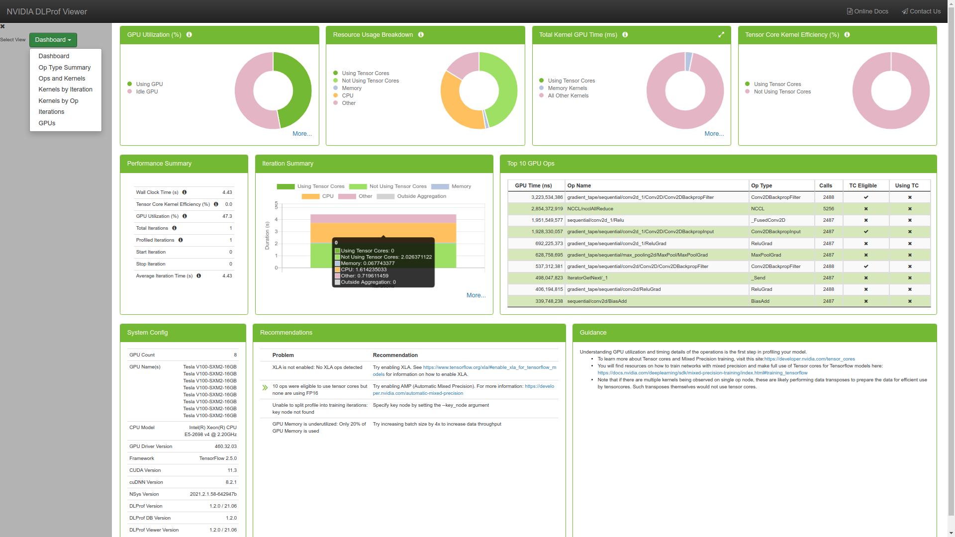
"You should be seeing the following page , this is called the DLProf Dashboard. The Dashboard view provides a high level summary of the performance results in a panelized view. This view serves as a starting point in analyzing the results and provides several key metrics.\n",
"\n",
"**Note** : If you are not able to access the DLProf dashboard , kindly verify if you have access to port and verify if the port number forwarded matches the port dlprofviewer server is running on.\n",
"\n",
"\n",
"\n",
"Let us now focus on the Dashboard and understand what the differnet panels in the Dashboard are for.\n",
"\n",
"- **GPU Utilization Chart**: Shows the percentage of the wall clock time that the GPU is active. For multi-gpu, it is an average utilization across all GPUs\n",
"- **Op GPU Time Chart**: Splits all operations into 3 categories: Operations that used tensor cores, operations that were eligible to use tensor cores but didn't, and operations that were ineligible to use tensor cores\n",
"- **Kernel GPU Time Chart**: Breaks down all kernel time into 3 categories: Kernels that used tensor cores, memory kernels, and all other kernels\n",
"- **Tensor Core Kernel Efficiency Chart**: Gives a single number that measures what percentage of GPU time inside of TC-eligible ops are using tensor cores. \n",
"- **Performance summary**: A straightforward panel that shows all of the key metrics from the run in one place\n",
"- **Iteration Summary**: A bar chart that shows the amount of time each iteration took during the run. The colored bars are the ones that were used to generate all of the statistics, while the gray bars are iterations that were outside the selected range. Each colored bar shows the breakdown of iteration time into GPU using TC, GPU not using TC, and all other non-GPU time.\n",
"- **Top 10 GPU Ops**: Shows the top 10 operations in the run sorted by the amount of GPU time they took. This is a great starting point for trying to find potential for improvements \n",
"- **System Config**: Shows the system configuration for the run.\n",
"- **Expert Systems Recommendations**: Shows any potential problems that DLProf found and recommendations for how to fix them.\n",
"- **Guidance Panel**: Provides some helpful links to learn more about GPU utilization and performance improvements\n",
"\n",
"\n",
"Let us now look at some more details provided by the DLProf Viewer \n",
"\n",
"\n",
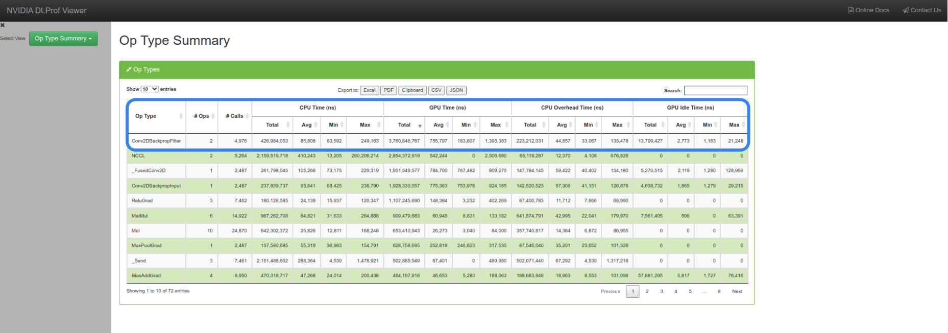
"**Op Type Summary** : This page contains tables that aggregates metrics over all op types and enables users to see the performance of all the ops in terms of its types, such as Convolutions, Matrix Multiplications, etc.\n",
"\n",
"\n",
"\n",
"In the above image we can notice the tabular data is sorted by the time taken by the GPU for every operation. This allows us to understand the number of times an operation is called and the time taken by them , this will be used in the System Topology notebook to differentiate between the different types of GPU-GPU connectivity.\n",
"\n",
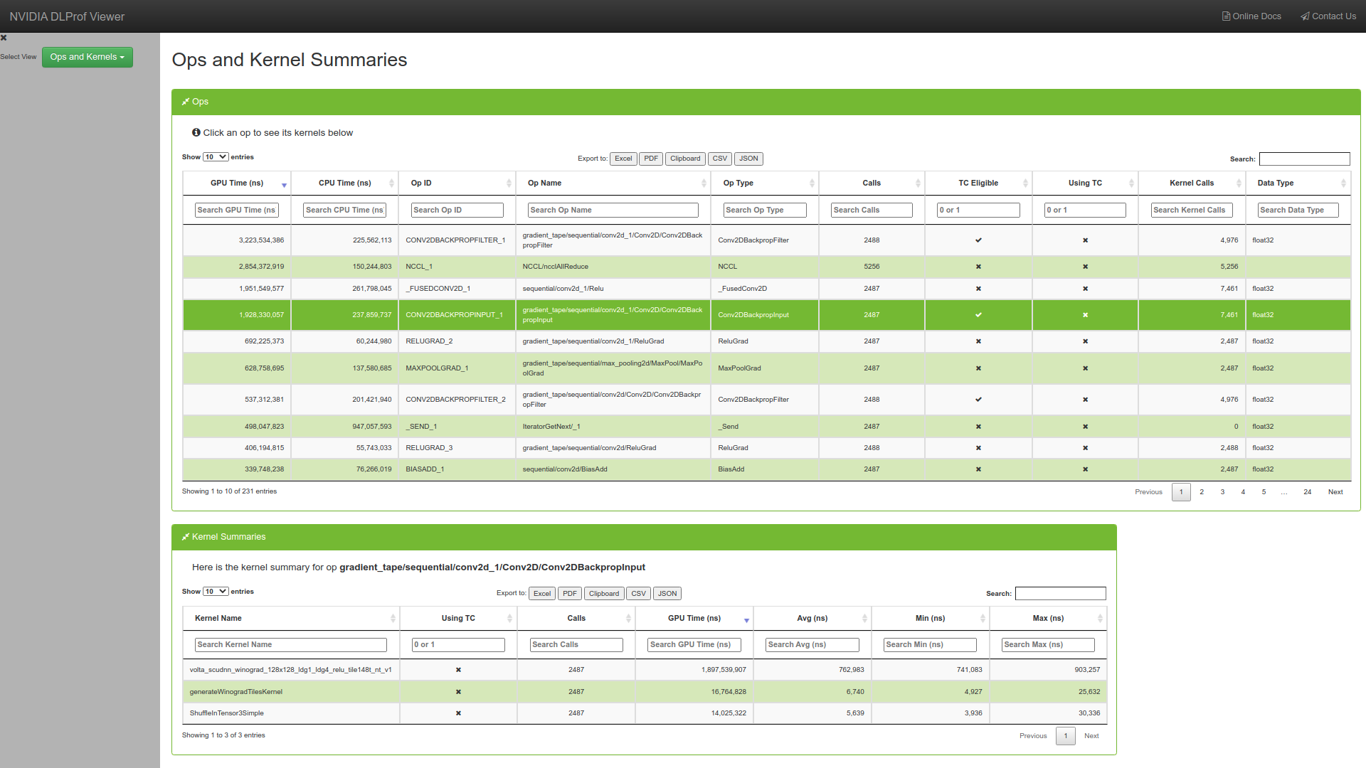
"**Ops and Kernels** : This view enables users to view, search, sort all ops and their corresponding kernels in the entire network.\n",
"\n",
"\n",
"\n",
"We will look into the remaining tabs in the following section.\n",
"\n",
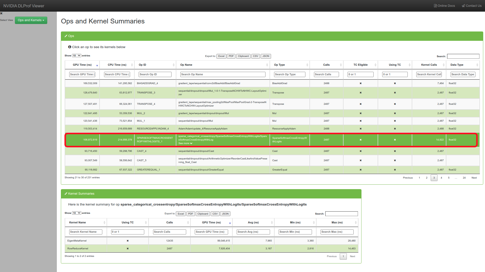
"Let us now profile again with `key_node` parameter , remember the `key_node` parameters is used to define a iteration , so we need to look for an operation in the **Ops and Kernels Summary** tab that occurs at every iteration.\n",
"\n",
"Here , let us choose the loss function operation name as `key_node` as we are aware this is calculated at the end of every iteration.\n",
"\n",
"\n",
"\n",
"\n",
"Let us now add this parameter to profile our deep learning workload.\n",
"\n",
"```bash\n",
"--key_node=sparse_categorical_crossentropy/SparseSoftmaxCrossEntropyWithLogits/SparseSoftmaxCrossEntropyWithLogits\n",
"```\n",
"\n"
]
},
{
"cell_type": "code",
"execution_count": null,
"metadata": {},
"outputs": [],
"source": [
"!TF_CPP_MIN_LOG_LEVEL=3 dlprof --mode=tensorflow2 --key_node=sparse_categorical_crossentropy/SparseSoftmaxCrossEntropyWithLogits/SparseSoftmaxCrossEntropyWithLogits --output_path=\"Profile/Prof2\" horovodrun -np 1 python3 ../source_code/N1/cnn_fmnist.py --batch-size=2048"
]
},
{
"cell_type": "markdown",
"metadata": {},
"source": [
"Close the already running `dlprofviewer` server and run it again with the latest profile. \n",
"\n",
"```bash\n",
"dlprofviewer -b 0.0.0.0 -p 8000 Profile/Prof2/dlprof_dldb.sqlite\n",
"```"
]
},
{
"cell_type": "markdown",
"metadata": {},
"source": [
"We again come across the Dashboard , but this time we will be having a different Dashboard compared the the previous one as we have added the `key_node` parameter thus defining an iteration. This allows us to compare multiple parameters between different iterations. \n",
"\n",
"Here's a short brief on the remaining tabs that utilise the `key_node` parameter to display information tagged with iterations : \n",
"\n",
"- **Kernels by Iteration** : The Kernels by Iterations view shows operations and their execution time for every iteration. At a glance, you can compare iterations with respect to time as well as Kernels executed.\n",
"\n",
"- **Kernels by Op** : The Kernels by Op view is a variation of the Kernels by Iterations view. It has the capability to filter the list of kernels by iterations and op.\n",
"\n",
"- **Iterations** : This view displays iterations visually. Users can quickly see how many iterations are in the model, the iterations that were aggregated/profiled, and the accumulated durations of tensor core kernels in each iteration.\n",
"\n",
"Here is an example of the iterations tab where we have access to information specific to each iteration of training : \n",
"\n",
"
\n",
"\n",
"and run the following command to launch the `dlprofviewer` server with the port `8000` . Kindly change it to a port that you will be using. \n",
"\n",
"```bash\n",
"dlprofviewer -b 0.0.0.0 -p 8000 /Profile/Prof1/dlprof_dldb.sqlite\n",
"```\n",
"\n",
"You should now have a `dlprofviewer` server running on the port specific. \n",
"\n",
"Open a new tab in your browser and navigate to `127.0.0.1:8000` to access the `dlprofviewer` application. You need to change the port number here to the one you specified while launching the server. \n",
"\n",
"You should be seeing the following page , this is called the DLProf Dashboard. The Dashboard view provides a high level summary of the performance results in a panelized view. This view serves as a starting point in analyzing the results and provides several key metrics.\n",
"\n",
"**Note** : If you are not able to access the DLProf dashboard , kindly verify if you have access to port and verify if the port number forwarded matches the port dlprofviewer server is running on.\n",
"\n",
"\n",
"\n",
"Let us now focus on the Dashboard and understand what the differnet panels in the Dashboard are for.\n",
"\n",
"- **GPU Utilization Chart**: Shows the percentage of the wall clock time that the GPU is active. For multi-gpu, it is an average utilization across all GPUs\n",
"- **Op GPU Time Chart**: Splits all operations into 3 categories: Operations that used tensor cores, operations that were eligible to use tensor cores but didn't, and operations that were ineligible to use tensor cores\n",
"- **Kernel GPU Time Chart**: Breaks down all kernel time into 3 categories: Kernels that used tensor cores, memory kernels, and all other kernels\n",
"- **Tensor Core Kernel Efficiency Chart**: Gives a single number that measures what percentage of GPU time inside of TC-eligible ops are using tensor cores. \n",
"- **Performance summary**: A straightforward panel that shows all of the key metrics from the run in one place\n",
"- **Iteration Summary**: A bar chart that shows the amount of time each iteration took during the run. The colored bars are the ones that were used to generate all of the statistics, while the gray bars are iterations that were outside the selected range. Each colored bar shows the breakdown of iteration time into GPU using TC, GPU not using TC, and all other non-GPU time.\n",
"- **Top 10 GPU Ops**: Shows the top 10 operations in the run sorted by the amount of GPU time they took. This is a great starting point for trying to find potential for improvements \n",
"- **System Config**: Shows the system configuration for the run.\n",
"- **Expert Systems Recommendations**: Shows any potential problems that DLProf found and recommendations for how to fix them.\n",
"- **Guidance Panel**: Provides some helpful links to learn more about GPU utilization and performance improvements\n",
"\n",
"\n",
"Let us now look at some more details provided by the DLProf Viewer \n",
"\n",
"\n",
"**Op Type Summary** : This page contains tables that aggregates metrics over all op types and enables users to see the performance of all the ops in terms of its types, such as Convolutions, Matrix Multiplications, etc.\n",
"\n",
"\n",
"\n",
"In the above image we can notice the tabular data is sorted by the time taken by the GPU for every operation. This allows us to understand the number of times an operation is called and the time taken by them , this will be used in the System Topology notebook to differentiate between the different types of GPU-GPU connectivity.\n",
"\n",
"**Ops and Kernels** : This view enables users to view, search, sort all ops and their corresponding kernels in the entire network.\n",
"\n",
"\n",
"\n",
"We will look into the remaining tabs in the following section.\n",
"\n",
"Let us now profile again with `key_node` parameter , remember the `key_node` parameters is used to define a iteration , so we need to look for an operation in the **Ops and Kernels Summary** tab that occurs at every iteration.\n",
"\n",
"Here , let us choose the loss function operation name as `key_node` as we are aware this is calculated at the end of every iteration.\n",
"\n",
"\n",
"\n",
"\n",
"Let us now add this parameter to profile our deep learning workload.\n",
"\n",
"```bash\n",
"--key_node=sparse_categorical_crossentropy/SparseSoftmaxCrossEntropyWithLogits/SparseSoftmaxCrossEntropyWithLogits\n",
"```\n",
"\n"
]
},
{
"cell_type": "code",
"execution_count": null,
"metadata": {},
"outputs": [],
"source": [
"!TF_CPP_MIN_LOG_LEVEL=3 dlprof --mode=tensorflow2 --key_node=sparse_categorical_crossentropy/SparseSoftmaxCrossEntropyWithLogits/SparseSoftmaxCrossEntropyWithLogits --output_path=\"Profile/Prof2\" horovodrun -np 1 python3 ../source_code/N1/cnn_fmnist.py --batch-size=2048"
]
},
{
"cell_type": "markdown",
"metadata": {},
"source": [
"Close the already running `dlprofviewer` server and run it again with the latest profile. \n",
"\n",
"```bash\n",
"dlprofviewer -b 0.0.0.0 -p 8000 Profile/Prof2/dlprof_dldb.sqlite\n",
"```"
]
},
{
"cell_type": "markdown",
"metadata": {},
"source": [
"We again come across the Dashboard , but this time we will be having a different Dashboard compared the the previous one as we have added the `key_node` parameter thus defining an iteration. This allows us to compare multiple parameters between different iterations. \n",
"\n",
"Here's a short brief on the remaining tabs that utilise the `key_node` parameter to display information tagged with iterations : \n",
"\n",
"- **Kernels by Iteration** : The Kernels by Iterations view shows operations and their execution time for every iteration. At a glance, you can compare iterations with respect to time as well as Kernels executed.\n",
"\n",
"- **Kernels by Op** : The Kernels by Op view is a variation of the Kernels by Iterations view. It has the capability to filter the list of kernels by iterations and op.\n",
"\n",
"- **Iterations** : This view displays iterations visually. Users can quickly see how many iterations are in the model, the iterations that were aggregated/profiled, and the accumulated durations of tensor core kernels in each iteration.\n",
"\n",
"Here is an example of the iterations tab where we have access to information specific to each iteration of training : \n",
"\n",
" \n",
"\n",
"\n",
"\n",
"The final tab give us the summary of GPU Utilisation :\n",
"\n",
"- **GPUs** : This view shows the utilization of all GPUs during the profile run.\n",
"\n",
"
\n",
"\n",
"\n",
"\n",
"The final tab give us the summary of GPU Utilisation :\n",
"\n",
"- **GPUs** : This view shows the utilization of all GPUs during the profile run.\n",
"\n",
" \n",
"\n",
"Now that we understand the types of information that DLProf provides us with , let us now take a look on how to improve our throughput using DLProf."
]
},
{
"cell_type": "markdown",
"metadata": {},
"source": [
"## Improving throughput using DLProf Expert system\n",
"\n",
"Until now we understand the amount of information made available to us via DLProf , but for an user trying to optimize their model and make use of new techniques, this information would not be straighforward , in that case the Expert Systems Recommendations is very helpful to find potential problems and recommendations for how to fix them.\n",
"\n",
"Let us take a closer look from the above profile.\n",
"\n",
"
\n",
"\n",
"Now that we understand the types of information that DLProf provides us with , let us now take a look on how to improve our throughput using DLProf."
]
},
{
"cell_type": "markdown",
"metadata": {},
"source": [
"## Improving throughput using DLProf Expert system\n",
"\n",
"Until now we understand the amount of information made available to us via DLProf , but for an user trying to optimize their model and make use of new techniques, this information would not be straighforward , in that case the Expert Systems Recommendations is very helpful to find potential problems and recommendations for how to fix them.\n",
"\n",
"Let us take a closer look from the above profile.\n",
"\n",
" \n",
"\n",
"Now that we have learnt the basics of DLProf and how to improve throughput using the DLProf expert systems.Let us now go back to the System topology notebook to use DLProf to understand the difference in communication times taken in different cases."
]
},
{
"cell_type": "markdown",
"metadata": {},
"source": [
"***\n",
"\n",
"## Licensing\n",
"\n",
"This material is released by OpenACC-Standard.org, in collaboration with NVIDIA Corporation, under the Creative Commons Attribution 4.0 International (CC BY 4.0)."
]
},
{
"cell_type": "markdown",
"metadata": {},
"source": [
"\n",
"\n"
]
}
],
"metadata": {
"kernelspec": {
"display_name": "Python 3",
"language": "python",
"name": "python3"
},
"language_info": {
"codemirror_mode": {
"name": "ipython",
"version": 3
},
"file_extension": ".py",
"mimetype": "text/x-python",
"name": "python",
"nbconvert_exporter": "python",
"pygments_lexer": "ipython3",
"version": "3.8.10"
}
},
"nbformat": 4,
"nbformat_minor": 4
}
\n",
"\n",
"Now that we have learnt the basics of DLProf and how to improve throughput using the DLProf expert systems.Let us now go back to the System topology notebook to use DLProf to understand the difference in communication times taken in different cases."
]
},
{
"cell_type": "markdown",
"metadata": {},
"source": [
"***\n",
"\n",
"## Licensing\n",
"\n",
"This material is released by OpenACC-Standard.org, in collaboration with NVIDIA Corporation, under the Creative Commons Attribution 4.0 International (CC BY 4.0)."
]
},
{
"cell_type": "markdown",
"metadata": {},
"source": [
"\n",
"\n"
]
}
],
"metadata": {
"kernelspec": {
"display_name": "Python 3",
"language": "python",
"name": "python3"
},
"language_info": {
"codemirror_mode": {
"name": "ipython",
"version": 3
},
"file_extension": ".py",
"mimetype": "text/x-python",
"name": "python",
"nbconvert_exporter": "python",
"pygments_lexer": "ipython3",
"version": "3.8.10"
}
},
"nbformat": 4,
"nbformat_minor": 4
}